Modern art using the GPU

I give you the same question Neo got; do you take the red pill or do you take the blue pill? After studying the Mandelbrot set, the complexity, rich and beauty of a simple definition, the endless iteration of a function, it will suck you into a world of fractals.

Again, we welcome Iterated Function Systems, whom will help us generate the Mandelbrot set. The Mandelbrot is simply just a group of numbers that display properties, and is based on iterated functions on a complex plane (see tutorial 1). In other words, the Mandelbrot set is a visual representations of an iterated function on the complex plane.

Let’s take a look at the Mandelbrot set:

It got a few inner black bulbs with a nice and REALLY complex pattern of pears around them. The complexity of the pattern can be seen below:

Basically, you can dive deep into the pattern of this border, without ever reaching the end, it’s and infinite complex pattern, a fractal curve.

So how is it possible that a simple function produces something like this? Let’s start with the function:

As you can see, this is an iterative function, where c is a complex number. This function takes z as the input, squares the input and adds a constant complex number c to it. Example: The functions starts with a value v, and generates the rest of the values using the previous v as the input:

As an example with actual data, lets try to calculate f(2).

We see that the output is getting really large at a fast pace. If we try to put in any number greater than 1, and less than –2, this will happen. But in between, something magical is happening.

This behavior is explained by squaring numbers. We know that when squaring a number less than one, we will get a smaller number, so 0,2*0,2 is 0,04. So iterating this will decrease the output of the squaring, plus the value in c, increasing the output with smaller and smaller amounts. You can actually iterate this function without ever getting the result of 1.

Next, from tutorial 1, we know that all negative numbers have positive squares.

Lets take another look at our complex plane, using the function .

As the real number grows outside –2 and 1, any imaginary number will grow outside –2i and 2i. On other words, all imaginary numbers inside the red circle do not grow. These numbers are called the M-Set.

The red circle is showing all possible numbers within the Mandelbrot set, where the output after the first iteration, is still inside. Let’s give all these numbers that are still inside after the first iteration a color of blue. Now we got one circle of blue like the one above. Doing another iteration, let’s color all of the numbers that fall outside the blue circle yellow. Now we got a blue circle with a yellow circle inside. Again, after the next iteration, we color the numbers that fall outside the yellow circle another color, and then we continue this way untill we have reached the desired iteration.

We can see that our fractal becomes more and more detailed for every iteration we take. Normally, a really detailed Mandelbrot set requires a huge amount of iterations. The image you see above is the set all complex numbers c that produces a finite orbit of 0. If the point is not in M, it will explode (outside of –2 to 1 R, or –2 to 2 i).

Continuous coloring
In the image above, we have used an algorithm named escape time algorithm. This method for coloring our fractal creates bands of colors, like in the image above. The way this works is to count the amount if iterations before a point reaches the infinity, or the escape point. Typically, you use a dark color for the everything that falls outside our circle, and then increasing the brightness of this color for each iteration. But, we want to have a smooth and continuous color on our fractal.

In order to be able to have a smooth transition between the iterations, we can use an algorithm named Normalized Iteration Count. The formula for this is:

v(z) is a real number, where n is the iteration, z is x*x + y*y and N is 2.0.
For more information, visit the wikipedia page. This function outputs a number in the interval [0,1], and we can use this result in the color channels for rgb, scaling components as we want.

Implementing the Mandelbrot Set
Now that you know how the Mandelbrot works, let’s try and implement this.
The implementation is based on a HLSL pixel shader only, using DirectX 11.

In this example, nothing is done outside of the shader, except drawing a quad that fills the entire screen, and then pushing that quad through our vertex and pixel shader. The rest is up to the GPU and DirectX 11!

We start by defining the pixel shader:

float4 PS_Mandelbrot( PS_INPUT input) : SV_Target
{

}

Then we find the current position of the point we are going to work with, using the texture coordinates of our model. We store this in a variable named C, and another named v. These will be our starting values.

float4 PS_Mandelbrot( PS_INPUT input) : SV_Target
{
    float2 C = (input.Tex – 0.5)*4;
    float2 v = C;
}

Next, we must know how many iterations we want the fractal to go through, and we also define an index i that will contain the current iteration, starting from 0, and also another variable named prevIteration that will start with the highest iteration number.

float4 PS_Mandelbrot( PS_INPUT input) : SV_Target
{
    float2 C = (input.Tex – 0.5)*4;
    float2 v = C;

    int Iterations = 29;
    int prevIteration = Iteration;
    int i = 0;
}
Now, we will create the Mandelbrot value itself. This is done in a do/while loop, where we go through all of the iterations and calculate the Mandelbrot value:

float4 PS_Mandelbrot( PS_INPUT input) : SV_Target
{
    float2 C = (input.Tex – 0.5)*4;
    float2 v = C;

    int Iterations = 29;
    int prevIteration = Iterations;
    int i = 0;

    do
    {
        v = float2((v.x * v.x) – (v.y * v.y), v.x * v.y * 2) + C;
        i++;
        if ((prevIteration == Iterations) && ((v.x * v.x) + (v.y * v.y)) > 4.0)
        {
             prevIteration = i + 1;
        }
    }
    while (i < prevIteration);
}

Here, we calculate our point v with the previous content of v as the input, and then we add C. Can you see what function this is?

The last thing we do is to take the Mandelbrot value v, the iteration we are on and calculate the NIC (Normalized Iteration Count) using the following formula:

Now, we know that this function returns a number between 0 and 1. This can be used in a periodic function like sinus or cosnius. We can also scale the color in each RGB channel to get a nice looking color on our fractal. This is how our pixel shader so far:

float4 PS_Mandelbrot( PS_INPUT input) : SV_Target
{
float2 C = (input.Tex – 0.5)*4;
float2 v = C;

int Iterations = 29;
int prevIteration = Iterations;
int i = 0;

do
{
v = float2((v.x * v.x) – (v.y * v.y), v.x * v.y * 2) + C;

i++;

if ((prevIteration == Iterations) && ((v.x * v.x) + (v.y * v.y)) > 4.0)
{
prevIteration = i + 1;
}
}
while (i < prevIteration);

float NIC = (float(i) – (log(log(sqrt((v.x * v.x) + (v.y * v.y)))) / log(2.0))) / float(Iterations);
return float4(sin(NIC * Color.x), sin(NIC * Color.y), sin(NIC * Color.z), 1);
}

We still need to be able to control our movement in the fractal. Right now, compiling and running this will render a good looking fractal from a distance, with no movement.

To add movement, all we need to do is to modify this line of code:

float2 C = (input.Tex – 0.5)*4;

C will be used as our constant C, and is a 2d coordinate. It contains the position of the pixel we are working on. Now, if we add a few parameters to our shader, we can start using these to control C.

float2 Pan;
float Zoom;
float Aspect;

Pan will be used for moving left, right, up and down, zoom will be used to move in or out of the fractal, and aspect will be used as the aspect ratio for our fractal. Taking these into our calculation, we end up with a line of code that look like this:
float2 C = (input.Tex – 0.5) * Zoom * float2(1, Aspect) – Pan;

..and while at it, let’s add another parameter for the number of Iterations as well.
The final shader looks like this:

//————————————————————————————–
// Constant Buffer Variables
//————————————————————————————–

cbuffer cbShaderParameters : register( b0 )
{
int Iterations;
float2 Pan;
float Zoom;
float Aspect;
float3 Color;
float dummy1;
int dummy2;
};

//————————————————————————————–
// Input structures
//————————————————————————————–
struct VS_INPUT
{
float4 C : POSITION;
float2 Tex : TEXCOORD0;
};

struct PS_INPUT
{
float4 C : SV_POSITION;
float2 Tex : TEXCOORD0;
};

//————————————————————————————–
// Vertex Shader
//————————————————————————————–
PS_INPUT VS( VS_INPUT input )
{
PS_INPUT output = (PS_INPUT)0;
output.C = input.C;
output.Tex = input.Tex;

return output;
}

//————————————————————————————–
// Pixel Shader
//————————————————————————————–
float4 PS_Mandelbrot( PS_INPUT input) : SV_Target
{
float2 C = (input.Tex – 0.5) * Zoom * float2(1, Aspect) – Pan;
float2 v = C;

int prevIteration = Iterations;
int i = 0;

do
{
v = float2((v.x * v.x) – (v.y * v.y), v.x * v.y * 2) + C;

i++;

if ((prevIteration == Iterations) && ((v.x * v.x) + (v.y * v.y)) > 4.0)
{
prevIteration = i + 1;
}
}
while (i < prevIteration);

float NIC = (float(i) – (log(log(sqrt((v.x * v.x) + (v.y * v.y)))) / log(2.0))) / float(Iterations);

return float4(sin(NIC * Color.x), sin(NIC * Color.y), sin(NIC * Color.z), 1);
}

And there we have a nice and beautiful Mandelbrot set. Be aware on your journeys through it, you might get lost

The above picture is rendered with 29 iterations. Let’s increase this to 515!

The amount of details increases, and you can move deep into it and still see the details.

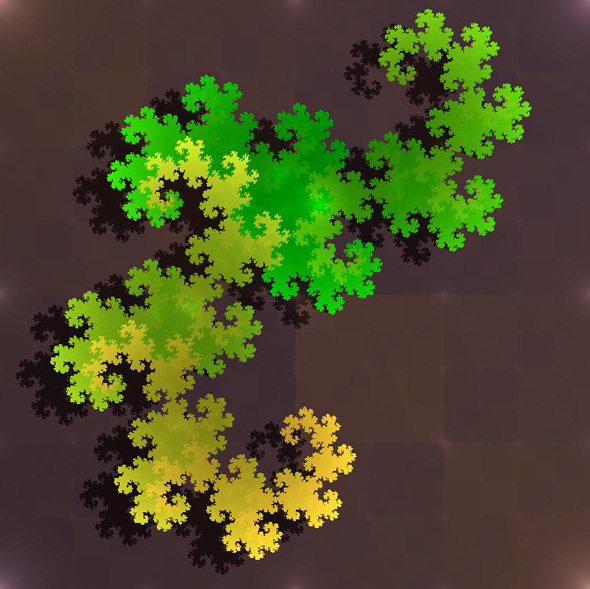
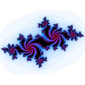
Examples
This is some images taken from my last trip into the world of the Mandelbrot Set:

Any feedback is welcome. I want to correct these and provide you guys with good tutorials.

Download: Source + Executable (DirextX11 + Visual Studio 2010)

The Sierpinski gasket is a fractal and a very basic fractal of self-similar sets, a mathematically generated pattern with similar patterns. The Sierpisnki gasket is typically generated using triangles, but you can render any shape you want in the space, and it’s an example of an iterated function system (IFS).

The Sierpinski gasket can be generated in many different ways. You can create a triangle, and cut out the parts that that’s not part of the Sierpinski gasket, or draw dots that after many plots, fill out the entire thing.

Programming your first fractal using dots
Implementing the Sierpinski gasket using dots is actually very simple. All you need to know is how to divide! You draw dots many at given positions, using the previous position as the input to the next position.

So, each point S_k is based in the previous point S_k-1.

Next we need to know what the function f(x) does, except for returning the coordinate of a point inside the Sierpinski gasket.
1. First of all, you need to select three points that form a triangle of any sort. These three points is defining the edges of the triangle:

Here we define point P0, P1 and P2 in a 2d coordinate system.

2. Next, use a random function to select any of the three points as a starting point. Let’s name this P_start.

3. Create the next point S_k as the midpoint between a random edge point P and the previous point S_k-1:

4. Draw S_k.

5. Jump to step 3

After a few iterations, this is what you will see:

S1 is the midpoint between P0 and P1, S2 is the midpoint between S1 and P2, and S3 is the midpoint between S2 and P1.

Implementing the Sierpinski gasket in DirectX 11
First, we need to define the edges of the Sierpinski gasket:

XMFLOAT2 EdgePoints[3];
EdgePoints[0].x = 0;
EdgePoints[0].y = 100;

EdgePoints[1].x = -100;
EdgePoints[1].y = -100;

EdgePoints[2].x = 100;
EdgePoints[2].y = -100;

Here, we create a triangle that is looking like the one in the figure above, it’s 200 wide and 200 high, ranging from –100 to 100 on both the x- and the y-axis.

Next, we need to select one of the edgepoints P at random:

int index = rand()%3;
XMFLOAT2 StartPoint = EdgePoints[index];
SierpinskiPoints[0] = StartPoint;

In the code above, we use a random-function as the lookup value into our edge points, grab the coordinate and store it in an array named SierpinkiPoints as the first element. This array will contain all our points, including the start coordinate. This means that this array will need to have the same size as how many dots we want to draw our Sierpinski gasket with.

Then we need to calculate the rest of the points:

for(int i = 1; i < Iterations; i++)
{
    index = rand()%3;
    StartPoint.x = (StartPoint.x + EdgePoints[index].x)/2.0f;
    StartPoint.y = (StartPoint.y + EdgePoints[index].y)/2.0f;
    SierpinskiPoints[i] = StartPoint;
}

Here, we will loop through step 3 to step 5 “Iterations” number of times, starting from element 1 as 0 is the starting point we created earlier. Then we select another random starting point and calculate the midpoint between the previous point that exist in StartPoint and the randomly selected EdgePoint. After that, we store our point in the SierpinskiPoints array and continue with the next point until all Iterations have been processed.
And that’s it, all we need to do now is do render all the points in the SierpinskiPoints array. But first, let’s take a look at the entire function we just wrote:

// Sierpinski gasket
const int Iterations = 20000;
XMFLOAT2 SierpinskiPoints[Iterations];

void BuildSierpinski()
{
    XMFLOAT2 EdgePoints[3];
    EdgePoints[0].x = 0;
    EdgePoints[0].y = 100;

    EdgePoints[1].x = -100;
    EdgePoints[1].y = -100;

    EdgePoints[2].x = 100;
    EdgePoints[2].y = -100;

    int index = rand()%3;
    XMFLOAT2 StartPoint = EdgePoints[index];
    SierpinskiPoints[0] = StartPoint;

    for(int i = 1; i < Iterations; i++)
    {
        index = rand()%3;
        StartPoint.x = (StartPoint.x + EdgePoints[index].x)/2.0f;
        StartPoint.y = (StartPoint.y + EdgePoints[index].y)/2.0f;
        SierpinskiPoints[i] = StartPoint;
    }

}

I’m using a square as the dot that will be rendered at every point in the SierpinskiPoints array.

// Clear the back buffer
float ClearColor[4] = { 0.33f, 0.4235f, 0.0627f, 1.0f }; // red,green,blue,alpha
g_pImmediateContext->ClearRenderTargetView( g_pRenderTargetView, ClearColor );
g_pImmediateContext->ClearDepthStencilView( g_pDepthStencilView, D3D11_CLEAR_DEPTH, 1.0f, 0 );

// Render our startpoint
g_World1 = XMMatrixScaling( 0.5f, 0.5f, 0.5f ) * XMMatrixTranslation( SierpinskiPoints[0].x, SierpinskiPoints[0].y, 0.0f );

CBShaderParameters cb1;
cb1.mWorld = XMMatrixTranspose( g_World1 );
cb1.mView = XMMatrixTranspose( g_View );
cb1.mProjection = XMMatrixTranspose( g_Projection );
g_pImmediateContext->UpdateSubresource( g_pCBShaderParameters, 0, NULL, &cb1, 0, 0 );

// Render a triangle
g_pImmediateContext->VSSetShader( g_pVertexShader, NULL, 0 );
g_pImmediateContext->VSSetConstantBuffers( 0, 1, &g_pCBShaderParameters );
g_pImmediateContext->PSSetShader( g_pPixelShader, NULL, 0 );
g_pImmediateContext->PSSetConstantBuffers( 0, 1, &g_pCBShaderParameters );
g_pImmediateContext->UpdateSubresource( g_pCBShaderParameters, 0, NULL, &cb1, 0, 0 );
g_pImmediateContext->Draw( 3, 0 );

for(int i = 1; i < Iterations; i++)
{
    g_World1 =  XMMatrixScaling( 0.5f, 0.5f, 0.5f ) * XMMatrixTranslation( SierpinskiPoints[i].x, SierpinskiPoints[i].y, 0.0f );

    CBShaderParameters cb1;
    cb1.mWorld = XMMatrixTranspose( g_World1 );
    cb1.mView = XMMatrixTranspose( g_View );
    cb1.mProjection = XMMatrixTranspose( g_Projection );
    g_pImmediateContext->UpdateSubresource( g_pCBShaderParameters, 0, NULL, &cb1, 0, 0 );

    // Render a triangle
    g_pImmediateContext->VSSetShader( g_pVertexShader, NULL, 0 );
    g_pImmediateContext->VSSetConstantBuffers( 0, 1, &g_pCBShaderParameters );
    g_pImmediateContext->PSSetShader( g_pPixelShader, NULL, 0 );
    g_pImmediateContext->PSSetConstantBuffers( 0, 1, &g_pCBShaderParameters );
    g_pImmediateContext->UpdateSubresource( g_pCBShaderParameters, 0, NULL, &cb1, 0, 0 );
    g_pImmediateContext->Draw( 6, 0 );
}

All we do here is to first transform our first quad to the first point in the SierpinskiPoints array, the starting point, and draw the quad at this position. Next we iterate through the entire array, transforming and drawing each quad at it’s position in the Sierpinski gasket.

The result will be a Sierpinski gasket created entirely with dots:

You could also create this in a pixel shader, where you evaluate if every point on the screen is inside the Sierpinski or not.

Download: Source and executable (DirectX11, Visual Studio 2010)

Any feedback is very welcome, and please tell me if there are any mistakes here!